🪶 Bird Species - Image Classification using ML

Motivated Data Science and Machine Learning enthusiast.
Introduction
To be completely honest, I have no particular interest in birds. There are people who do like to admire their beauty and are willing to spend hours looking at encyclopedia's, trying to memorize the different species of the warm-blooded vertebrate's. However, I would rather be spending my afternoon's browsing through the latest chapter's of 'My Hero Academia' or binging through the awesomeness of Hajime Isayama's work in 'Attack on Titan'.
However, we all have that one cute girl in our class with the cutest hobbies and you bet when that hobby turns out to be bird watching, there is only one thing for you to do. Although, that is still not enough to make me look through that thick, dusty encyclopedia at the top of my book shelf that my aunt got me on my 8th birthday. So, I did what any other machine learning enthusiast would have done. Build a model and have it learn the different species of birds in my place.
Getting Started
Now that we have established our motivation for this project, the next step is to get the data to train our model on. So, we start by browsing through 'Kaggle' to find the relevant dataset. The following dataset has 63604 images 400 different species of birds.
data: https://www.kaggle.com/gpiosenka/100-bird-species
Perfect!!!
Now, we have the relevant data for our model we can start towards making more sense of our data and processing it before we use it in our machine learning model.
1. Getting our data ready
First, we need to import few libraries and mount our drive to google colab where our data is stored. Also, we will be using GPU in our project. It can be selected from the Runtime tab in google colab and changing the Hardware Accelerator to GPU.
from google.colab import drive
import tensorflow as tf
import tensorflow_hub as hub
import pandas as pd
import numpy as np
import matplotlib.pyplot as plt

% matplotlib inline

drive.mount("/content/drive")
print("GPU", "Available" if tf.config.list_physical_devices("GPU") else "Not Available")
Now that we have our image dataset ready, the next step is to load our dataset into colab as a DataFrame so we can start working with it. To achieve that, we will be using the pandas library. Then we can use the .read_csv() function from the pandas library to create our desired dataframe.
import pandas as pd

birds_data = pd.read_csv("/content/drive/MyDrive/Birds Data/birds.csv")
birds_data.head()
This should load the filepaths for our images as a dataframe and store it in the variable birds_data which we can later access to perfom further manipulations on our data.
| index | class index | filepaths | labels | data set |
| 0 | 0 | train/ABBOTTS BABBLER/001.jpg | ABBOTTS BABBLER | train |
| 1 | 0 | train/ABBOTTS BABBLER/002.jpg | ABBOTTS BABBLER | train |
| 2 | 0 | train/ABBOTTS BABBLER/003.jpg | ABBOTTS BABBLER | train |
| 3 | 0 | train/ABBOTTS BABBLER/004.jpg | ABBOTTS BABBLER | train |
| 4 | 0 | train/ABBOTTS BABBLER/005.jpg | ABBOTTS BABBLER | train |
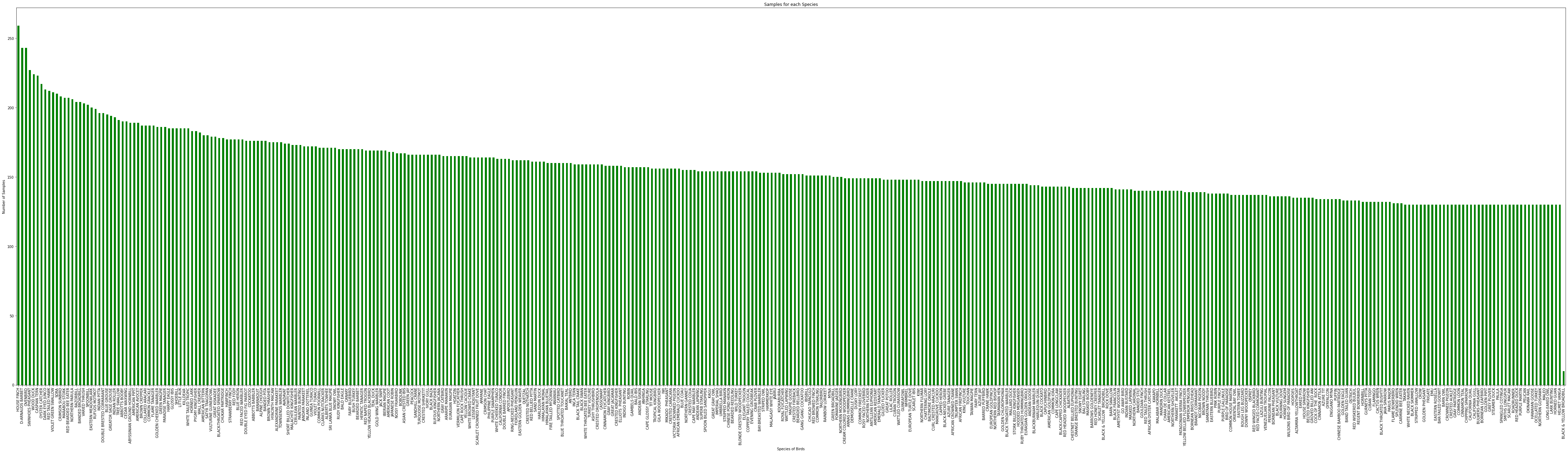
Now, let us visualize the number of samples that we have for each 400 species in our dataset using a bar graph.
plt.figure(figsize=(80,20))
plt.xlabel("Species of Birds")
plt.ylabel("Number of Samples")
plt.title("Samples for each Species")
birds_data.labels.value_counts().plot(kind="bar", color="green")
Below we can see the number of samples we have for each species in our dataset.
Let us get our labels ready!!!
For our model to predict the labels for our images we will be converting all of our labels into Boolean arrays of size 400.
#Creating Boolean Labels
boolean_labels = []
for i in range(len(birds_data)):
  boolean_labels.append(birds_data.labels[i] == birds_species)

labels = birds_data.labels
To easily access all the images in our dataset we will be creating a list of file paths for all the images.
#Creating File Paths
filepaths = []

for i in range(len(birds_data)):
  filepath = "/content/drive/MyDrive/Birds Data/" + str(birds_data.filepaths[i])
  filepaths.append(filepath)
2. Visualizing our data
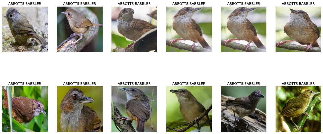
Now that we have our data prepared, let us visualize and see how the data that we are working with actually looks. We can do this by defining a function plot_image() that takes the list of file paths and the first and last index of the range of images that we want to be displayed.
#plot images
def plot_image(filepaths, start=0, end=12):
  """
  This function plots the images from a list of given filepaths.

  filepaths: List of the paths where the image is stored
  start: Starting index to plot the image from.
  end: Last index to plot the image to.
  """
  plt.figure(figsize=(20,30))
  rows = (end - start)//2
  cols = (end-start) - ((end - start)//2)

  for i in range(start, start + (end - start)):
    ax = plt.subplot(rows, cols, i+1-start)
    image = plt.imread(filepaths[i])
    plt.imshow(image)
    plt.title(birds_species[boolean_labels[i].argmax()])
    plt.axis("off")
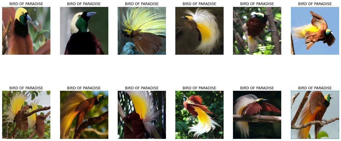
Now, let us look at some of the images from our dataset using our defined function plot_images().
plot_image(filepaths)
plot_image(filepaths, start=8400, end=8412)
3. Processing our data
Now that we have a better understanding of the data we are working with we need to perform certain pre-processing operations on our dataset before we can pass it to our model for learning.
#Define image size
IMG_SIZE = 224

# Create a function for preprocessing images
def process_image(image_path, img_size=IMG_SIZE):
  """
  Takes an image file path and turns the image into a Tensor.
  """
  # Read in an image file
  image = tf.io.read_file(image_path)
  # Turn the jpeg image into numerical Tensor with 3 colour channels (Red, Green, Blue)
  image = tf.image.decode_jpeg(image, channels=3)
  # Convert the colour channel values from 0-255 to 0-1 values
  image = tf.image.convert_image_dtype(image, tf.float32)
  # Resize the image to our desired value (224, 224)
  image = tf.image.resize(image, size=[IMG_SIZE, IMG_SIZE])

  return image
As our model requires us to pass the data in form of tensors, we define a function process_image() that takes the path of our image as input, converts it into tensors, resizes the image with width : 224,
height : 224 and color channels 3 (RGB) in the range(0,1) after normalization and returns the processed image.
We also define a helper function process_data() that returns a tuple of the processed image and its label.
#create a tuple of filepaths and labels
def process_data(filepath, label):
  image = process_image(filepath)
  return (image, label)
4. Creating data batches
To optimize the training process we need to create batches of our data to be passed to our model. Hence, we define a function create_batch() that will create batches of batch size 32 from our data depending on the type of data we pass to the function.
#creating data batches
BATCH_SIZE=32
def create_batch(filepaths, labels=None, test_data=False, valid_data=False):
  #Test Data
  if test_data == True:
    print("Creating test data batches......")
    dataset = tf.data.Dataset.from_tensor_slices(tf.constant(filepaths))
    data_batch = dataset.map(process_image).batch(BATCH_SIZE)

  elif valid_data == True:
    print("Creating validation data batches......")
    dataset = tf.data.Dataset.from_tensor_slices((tf.constant(filepaths),
                                                 tf.constant(labels)))
    data_batch = dataset.map(process_data).batch(BATCH_SIZE)


  else:
    print("Creating training data batches.........")
    dataset = tf.data.Dataset.from_tensor_slices((tf.constant(filepaths),
                                                tf.constant(labels)))

    dataset = dataset.shuffle(len(dataset))
    data_batch = dataset.map(process_data).batch(BATCH_SIZE)

  return data_batch
Now, let us create 3 different batches for training, validation and testing.
training_batch = create_batch(filepaths[:20000], boolean_labels[:20000])
validation_batch = create_batch(filepaths[:20000], boolean_labels[:20000], valid_data=True)
test_batch = create_batch(filepaths[:20000], boolean_labels[:20000], test_data=True)
As we will only be using the first 20,000 images from our dataset we have sliced our file paths and labels to only create batches of 20,000 images and labels.
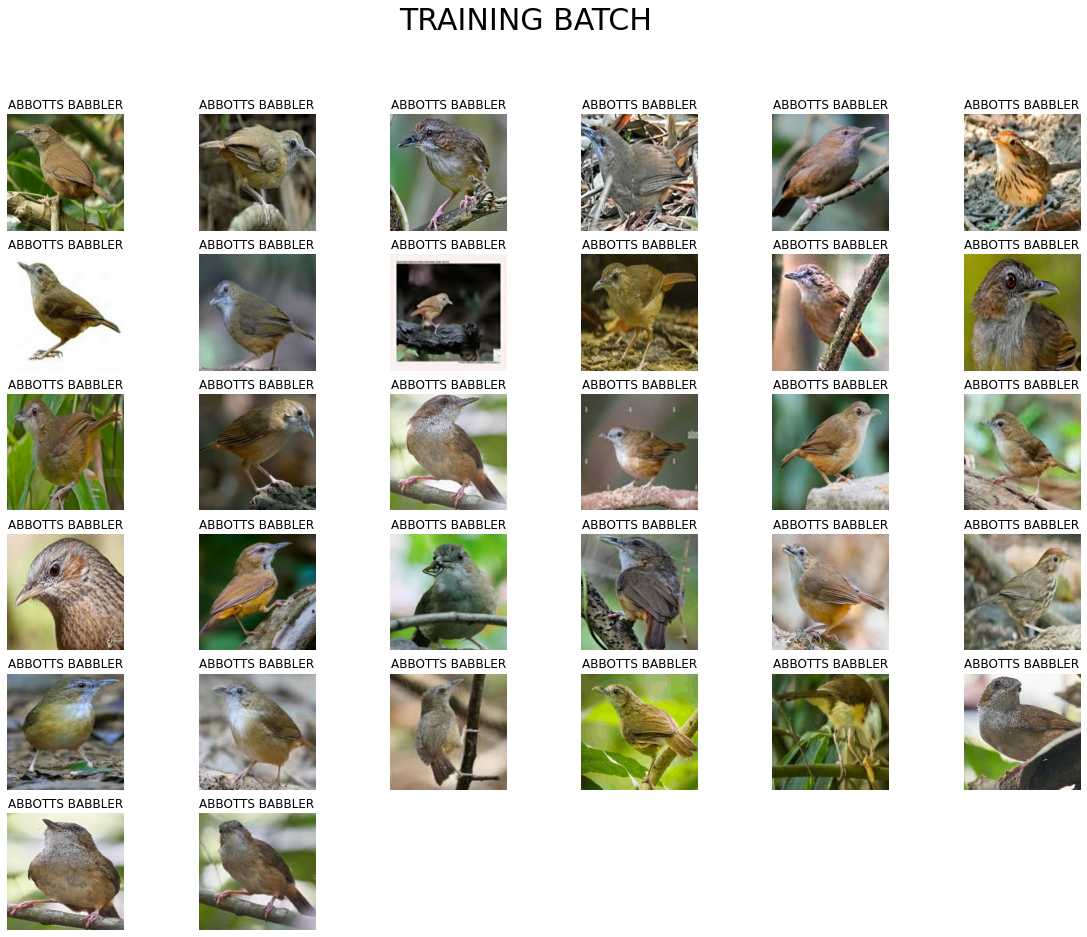
5. Visualizing data batch
Now that we have our data in batches let us define a function display_batch() to be able to see the images in our data batch.
#visualizing data batches
def display_batch(batch, valid_batch=False, test_batch=False):
  if test_batch == True:
    images = next(batch.as_numpy_iterator())
    plt.figure(figsize=(20,15))
    plt.suptitle("TEST BATCH", size=30)
    for i in range(len(images)):
      ax = plt.subplot(6,6, i+1)
      plt.imshow(images[i])
      plt.axis("off")

  elif valid_batch == True:
    images, labels = next(batch.as_numpy_iterator())
    plt.figure(figsize=(20,15))
    plt.suptitle("VALIDATION BATCH", size=30)
    for i in range(len(images)):
      ax = plt.subplot(6,6, i+1)
      plt.imshow(images[i])
      plt.title(birds_species[labels[i].argmax()])
      plt.axis("off")

  else:
    images, labels = next(batch.as_numpy_iterator())
    plt.figure(figsize=(20,15))
    plt.suptitle("TRAINING BATCH", size=30)
    for i in range(len(images)):
      ax = plt.subplot(6,6, i+1)
      plt.imshow(images[i])
      plt.title(birds_species[labels[i].argmax()])
      plt.axis("off")
Training Batch
display_batch(training_batch)
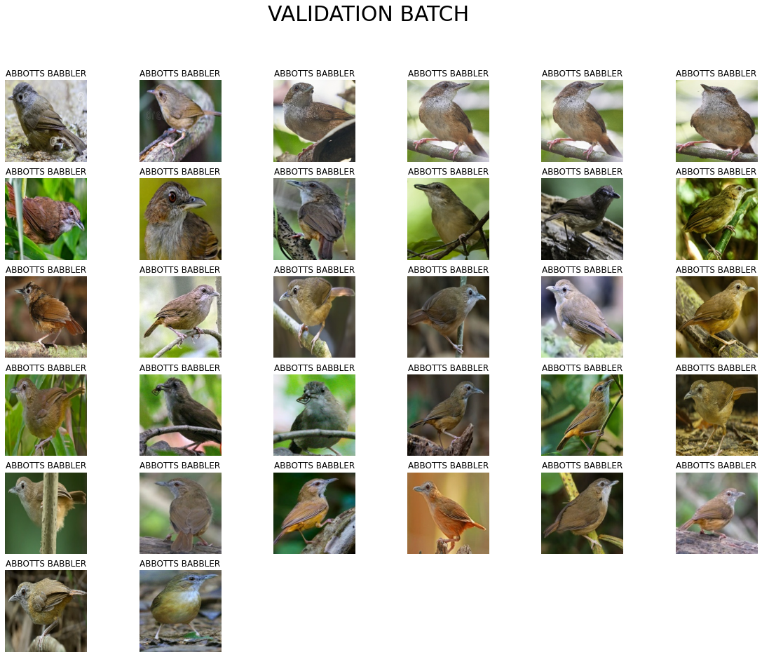
Validation Batch
display_batch(validation_batch, valid_batch=True)
Test Batch
display_batch(test_batch, test_batch=True)
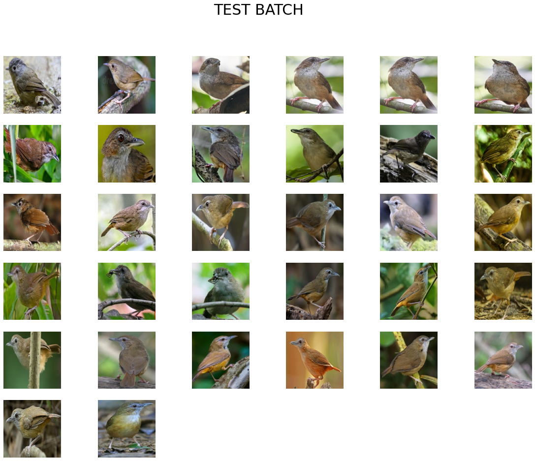
Notice how we don't have any labels for our test batch?
This is due to the fact that we will be having our trained model predict the labels for out testing batches.
6. Building our model
As we have performed the necessary pre-processing on our data and created batches to train our model on, let us start building our model.
First, we define the input shape of our data, the output shape and specify the model URL to be used.
INPUT_SHAPE = [None, 224, 224, 3]
OUTPUT_SHAPE = len(birds_species)
model_url = "https://tfhub.dev/tensorflow/efficientnet/b4/classification/1"
Then we define a function create_model() to create our model.
def create_model():
  model = tf.keras.Sequential([
                               hub.KerasLayer(model_url),
                               tf.keras.layers.Dense(OUTPUT_SHAPE,
                                                     activation=tf.nn.softmax)
  ])

  model.compile(
      optimizer=tf.keras.optimizers.Adam(),
      loss=tf.keras.losses.CategoricalCrossentropy(),
      metrics=["accuracy"]
  )

  model.build(INPUT_SHAPE)

  return model
Now that we have a function to create our model, let us define some callbacks for our model. We will be using the EarlyStopping and TensorBoard callback from the tf.Keras.Callbacks API.
#Creating Callbacks
import datetime
import os

#EarlyStopping
EarlyStopping = tf.keras.callbacks.EarlyStopping(monitor="accuracy",
                                                 patience=3)

#TensorBoard Callback
def create_TensorBoard():
  log_dir = "/content/drive/MyDrive/Birds Data/logs/" + datetime.datetime.now().strftime("%Y%m%d-%H%M%s")

  return tf.keras.callbacks.TensorBoard(log_dir)
Now, let us train our model!!!!!
model = create_model()
model.summary()

model.fit(
    train_batch,
    verbose="auto",
    epochs=NUM_EPOCHS,
    callbacks=[EarlyStopping, TensorBoard],
    validation_data=valid_batch,
    validation_steps=10
)
The output should look similar to the following.
Model: "sequential_5"
_________________________________________________________________
 Layer (type)                Output Shape              Param #
=================================================================
 keras_layer_5 (KerasLayer)  (None, 1000)              19466816

 dense_5 (Dense)             (None, 401)               401401

=================================================================
Total params: 19,868,217
Trainable params: 401,401
Non-trainable params: 19,466,816
_________________________________________________________________
Epoch 1/100
350/350 [==============================] - 111s 272ms/step - loss: 5.7350 - accuracy: 0.1259 - val_loss: 5.4902 - val_accuracy: 0.1688
Epoch 2/100
350/350 [==============================] - 55s 158ms/step - loss: 5.2874 - accuracy: 0.2115 - val_loss: 5.0995 - val_accuracy: 0.2219
Epoch 3/100
350/350 [==============================] - 56s 158ms/step - loss: 4.9429 - accuracy: 0.2452 - val_loss: 4.7946 - val_accuracy: 0.2344
Epoch 4/100
350/350 [==============================] - 55s 156ms/step - loss: 4.6676 - accuracy: 0.2797 - val_loss: 4.5431 - val_accuracy: 0.2719
Epoch 5/100
350/350 [==============================] - 56s 159ms/step - loss: 4.4373 - accuracy: 0.3105 - val_loss: 4.3287 - val_accuracy: 0.3094
Epoch 6/100
350/350 [==============================] - 55s 156ms/step - loss: 4.2379 - accuracy: 0.3298 - val_loss: 4.1393 - val_accuracy: 0.3250
7. Making prediction with the trained model
HURRAYYY!!!!
Now that our model has learned from the training batches let us use it make some prediction on our validation data and visualize those predictions.
predictions = model.predict(valid_batch)
predictions
Let us now compare these predictions with the true values. But to do that first we need to unbatch our validation data to be able to access the images and labels, so let us write a function unbatch_data() to do the same.
#Unbatch the validation data
def unbatch_data(data):
  images = []
  labels = []
  for image, label in data.unbatch().as_numpy_iterator():
    images.append(image)
    labels.append(label)

  return images, labels

val_images, val_labels = unbatch_data(valid_batch)
Now that we have our predicted values and true values let us define few functions to visualize our predictions and see their accuracy.
def plot_pred(prediction_probabilities, labels, images, index=1):
  plt.imshow(images[index])
  plt.xticks([])
  plt.yticks([])

  if labels[index].argmax() == prediction_probabilities[index].argmax():
    color="green"
  else:
    color="red"

  plt.title("{}  {:.2f}%  {}".format(birds_species[labels[index].argmax()],
                                    prediction_probabilities[index].max() * 100,
                                    birds_species[prediction_probabilities[index].argmax()]),
            color=color)


def plot_top_preds(prediction_probabilities, labels, images, index=1):

  top_preds = prediction_probabilities[index].argsort()[-10:][::-1]

  top_plot = plt.bar(np.arange(len(top_preds)),
            prediction_probabilities[index][top_preds],
            color="grey")

  plt.xticks(np.arange(len(top_preds)),
                       birds_species[top_preds],
             rotation="vertical")

  true_label = birds_species[labels[index].argmax()]
  top_pred_labels = birds_species[top_preds]

  if np.isin(true_label, top_pred_labels):
    top_plot[np.argmax(top_pred_labels == true_label)].set_color("green")
  else:
    pass


def plot_pred_batch(prediction_probabilities, labels, images, index=1):
  plt.figure(figsize=(40,20))

  i_start = index
  num_images=20
  num_rows = 5
  num_cols = 4

  for i in range(num_images):
    plt.subplot(num_rows, num_cols*2, 2*i+1)
    plot_pred(prediction_probabilities, labels, images, i_start+i)

    plt.subplot(num_rows, num_cols*2, 2*i+2)
    plot_top_preds(prediction_probabilities, labels, images, i_start+i)

  plt.show()

plot_pred_batch(predictions, val_labels, val_images, 1)
Now let us see our model in it's complete glory!!!
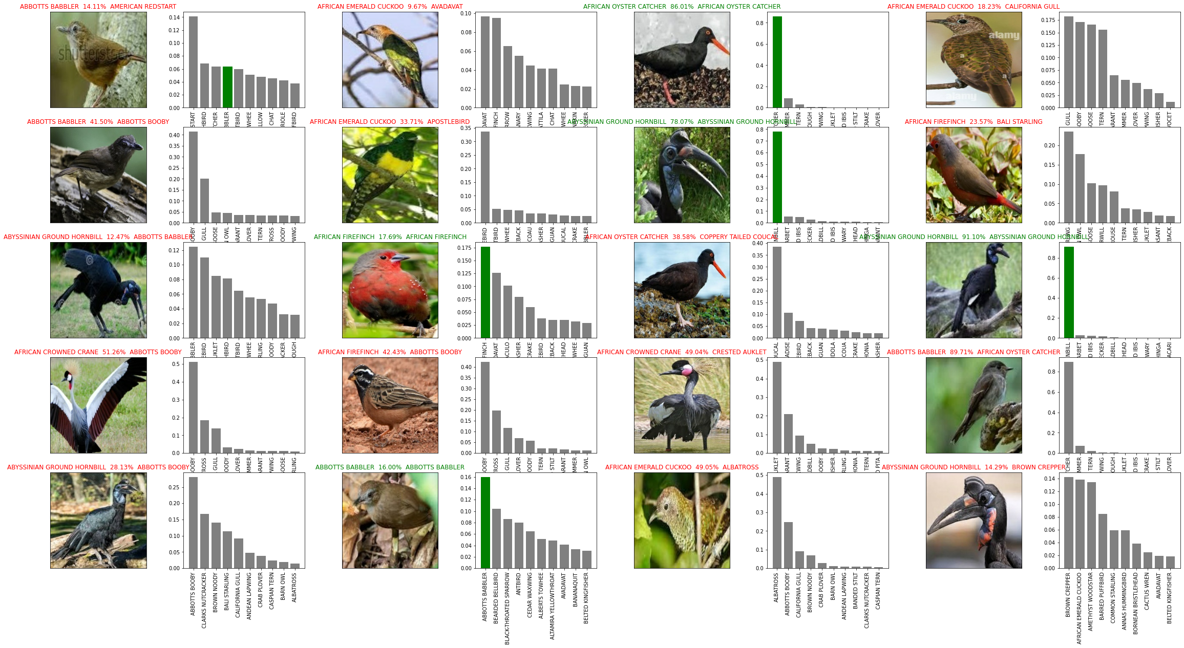
GREAT!!!
Now we have a working model to predict the species of bird.
We can further improve the accuracy of our model by increasing the sample size from 20,000 images or by using the entire datset of 63,604 images.
The end-to-end jupyter notebook for the project can be found below.
Github repo : https://github.com/Gitster7/Bird-Species-Image-Classification/blob/main/Bird_Species_Image_Classification.ipynb


